In order to effectively distribute the available telescope time and to maximize the overall timing precision, three main characteristics have to be considered: the aparent magnitude of the star, the size of the primary mirror, and the amplitude of the O-C diagram.

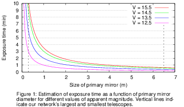
With the main goal to connect the KOIs to their most suitable telescopes, we proceeded as follows: first, we estimated the exposure time e_t for each star and telescope. This calculation was carried out considering parameters such as the mean seeing of the site, the brightness of the star, the desired signal-to-noise ratio, the size of the primary mirror, typical sky brightnesses, and the phase of the Moon and the altitude of the star during predicted observing windows, among others. We compared this estimations to real astronomical data, simply contrasting the exposure time, the size of the primary mirror, and the magnitude of the observed star obtained from the bibliography against our estimated cadence. Figure 1 shows our results, where the exposure time has been approximated with a power law of the telescope's diameter.

It is well known that off-transit data have a huge impact in the determination of the orbital and physical parameters of any transiting system. In the case of ground-based observations, off-transit data are critical to remove systematics such as airmass, color-dependent extinction, and poor guiding, among many others. Henceforth, to determine the number of data points N per transit we used the estimated exposure time and the known transit duration T_dur incremented by two hours. This increment accounts for 1 hour of off-transit data before and after transit begins and ends, respectively. Then, the number of data points N per transit was simply estimated as follows: N = (T_dur + 2)/e_t.

To estimate the timing precision σ_T we used a variant of the formulism provided by Ford & Holman (2007):

where T_depth is the transit depth, and Phot_prec is the photometric precision that a given telescope can achieve while observing a 14-15 K_mag star. This value was inquired to the members of KOINet at the beginning of the network's organization.

Comparing the estimated timing precision with the semi-amplitude of the O-C diagrams A_O-C (A_O-C > 3σ_T) jielded erroneous results, specially if the TTV was large (several hours). By instance, if the timing precision is determined as 1 hour, compared to a TTV amplitude of 3 hours the relation would be satisfied. But a timing precision of 1 hour is not only unrealistic but useless. Therefore, three aspects were simultaneously considered. Only if all of them where satisfied, then the KOI was assigned to the telescope. The aspects are the transit depth, the scatter of the O-C diagram, and its amplitude.

1) The transit depth is extremely relevant. Therefore, the first condition requires it to be larger than 75% the photometric precision that a given telescope can achieve observing Kepler kind-of stars, T_depth > 0.75 Phot_prec. To arrive to this value we made use of synthetic data: First, a primary transit light curve with duration comparable to a "normal" observing run (~6 hours) was produced. To this end, we made use of Mandel & Agol (2002) primary transit model. Then, white and correlated noise with amplitude comparable to Phot_prec was added. The cadence of the synthetic data was set to 3 minutes. Once the light curve was generated, the mid-transit time, semi-major axis, orbital inclination and transit depth were fitted to the synthetic data. Since Kepler light curves will provide accurate orbital parameters, this analysis will return overestimated error bars. This is in good agreement with our conservative approach. Figure 2 shows two synthetic primary transit light curves. The mean scatter of the data was set to 0.4% for the red one and 0.2% for the green one. In both cases the transit depth was set to 0.4%. To obtain the parameter estimates and their errors we have sampled from the posterior probability distribution using a Markov-chain Monte Carlo approach. For the fitted parameters we defined uniform priors covering a reasonable range. After 10⁶ iterations and an initial burn of 10⁵, the timing accuracy was obtained to be between 3 and 4 minutes for the red light curve and less than 2 minutes for the green one.

The previously mentioned limit between photometric precision and transit depth (i.e., T_depth > 0.75 Phot_prec) was obtained lowering the photometric precision of the synthetic light curves until a timing precision of 5 minutes was reached. This upper limit is considered to be competitive with Kepler timing precision and, for some cases, even better. For this analysis transit depths between 1% and 0.1% were considered.

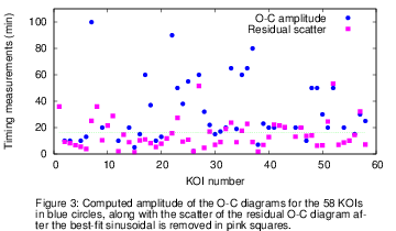
2) Closely analyzing the O-C diagrams we noticed that the computed amplitude was sometimes comparable to its scatter. This can be observed in Figure 3, where the amplitude of the observed TTVs (A_O-C) plotted in blue circles is compared to the scatter of the residual O-C diagram (pink squares) after the TTV variation was removed.

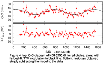
To better illustrate this we made use of a real system: KOI-0250. The top panel of Figure 4 shows the mid-transit times of the 17 quarters of Kepler data, overplotted with the best-fit sinusoidal modulation. The TTV amplitude was computed to be around 10 minutes. The bottom panel of the same Figure shows the residual timings once the TTV modulation was removed. In this case, the scatter of the residuals is comparable to the TTV amplitude. Since the errors of the individual mid-transit times could be underestimated (this is usually the case when systematic effects are not properly considered) we think a more conservative approach to consider the scatter of the residuals as overall timing precision. Since the O-C diagrams showing this behavior can return a proper dynamical description of a planetary system, our second condition relates the O-C amplitude and the timing precision as follows: A_O-C > σ_T.

3) Following the line of thought of Point 2), the third condition relates the scatter of the residual O-C diagrams σ_Kepler with the derived timing precision: 2σ_Kepler > σ_T.